Cryptocurrency Analysis with Python - Log Returns
In previous post, we analyzed raw price changes of cryptocurrencies. The problem with that approach is that prices of different cryptocurrencies are not normalized and we cannot use comparable metrics.
In this post, we describe benefits of using log returns for analysis of price changes. You can download this Jupyter Notebook and the data.
Follow me on twitter to get latest updates.
Here are a few links you might be interested in:
- Intro to Machine Learning
- Intro to Programming
- Data Science for Business Leaders
- AI for Healthcare
- Autonomous Systems
- Learn SQL
Disclosure: Bear in mind that some of the links above are affiliate links and if you go through them to make a purchase I will earn a commission. Keep in mind that I link courses because of their quality and not because of the commission I receive from your purchases. The decision is yours, and whether or not you decide to buy something is completely up to you.
Disclaimer
I am not a trader and this blog post is not a financial advice. This is purely introductory knowledge. The conclusion here can be misleading as we analyze the time period with immense growth.
Requirements
For other requirements, see my first blog post of this series.
Load the data
import pandas as pd

df_btc = pd.read_csv('BTC_USD_Coinbase_hour_2017-12-24.csv', index_col='datetime')
df_eth = pd.read_csv('ETH_USD_Coinbase_hour_2017-12-24.csv', index_col='datetime')
df_ltc = pd.read_csv('LTC_USD_Coinbase_hour_2017-12-24.csv', index_col='datetime')
df = pd.DataFrame({'BTC': df_btc.close,
                   'ETH': df_eth.close,
                   'LTC': df_ltc.close})
df.index = df.index.map(pd.to_datetime)
df = df.sort_index()
df.head()
| BTC | ETH | LTC | |
|---|---|---|---|
| 2017-10-02 08:00:00 | 4448.85 | 301.37 | 54.72 |
| 2017-10-02 09:00:00 | 4464.49 | 301.84 | 54.79 |
| 2017-10-02 10:00:00 | 4461.63 | 301.95 | 54.63 |
| 2017-10-02 11:00:00 | 4399.51 | 300.02 | 54.01 |
| 2017-10-02 12:00:00 | 4383.00 | 297.51 | 53.71 |
df.describe()
| BTC | ETH | LTC | |
|---|---|---|---|
| count | 2001.000000 | 2001.000000 | 2001.000000 |
| mean | 9060.256122 | 407.263793 | 106.790100 |
| std | 4404.269591 | 149.480416 | 89.142241 |
| min | 4150.020000 | 277.810000 | 48.610000 |
| 25% | 5751.020000 | 301.510000 | 55.580000 |
| 50% | 7319.950000 | 330.800000 | 63.550000 |
| 75% | 11305.000000 | 464.390000 | 100.050000 |
| max | 19847.110000 | 858.900000 | 378.660000 |
Why Log Returns?
Benefit of using returns, versus prices, is normalization: measuring all variables in a comparable metric, thus enabling evaluation of analytic relationships amongst two or more variables despite originating from price series of unequal values (for details, see Why Log Returns).
Let’s define return as:
\[r_{i} = \frac{p_i - p_j}{p_j},\]where $r_i$ is return at time $i$, $p_i$ is the price at time $i$ and $j = i-1$.
Calculate Log Returns
Author of Why Log Returns outlines several benefits of using log returns instead of returns so we transform returns equation to log returns equation:
\[r_{i} = \frac{p_i - p_j}{p_j}\] \[r_i = \frac{p_i}{p_j} - \frac{p_j}{p_j}\] \[1 + r_i = \frac{p_i}{p_j}\] \[log(1+r_i) = log(\frac{p_i}{p_j})\] \[log(1+r_i) = log(p_i) - log(p_j)\]Now, we apply the log returns equation to closing prices of cryptocurrencies:
import numpy as np

# shift moves dates back by 1
df_change = df.apply(lambda x: np.log(x) - np.log(x.shift(1)))
df_change.head()
| BTC | ETH | LTC | |
|---|---|---|---|
| 2017-10-02 08:00:00 | NaN | NaN | NaN |
| 2017-10-02 09:00:00 | 0.003509 | 0.001558 | 0.001278 |
| 2017-10-02 10:00:00 | -0.000641 | 0.000364 | -0.002925 |
| 2017-10-02 11:00:00 | -0.014021 | -0.006412 | -0.011414 |
| 2017-10-02 12:00:00 | -0.003760 | -0.008401 | -0.005570 |
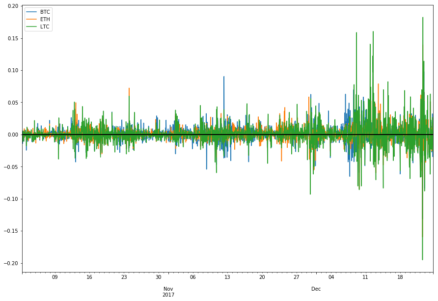
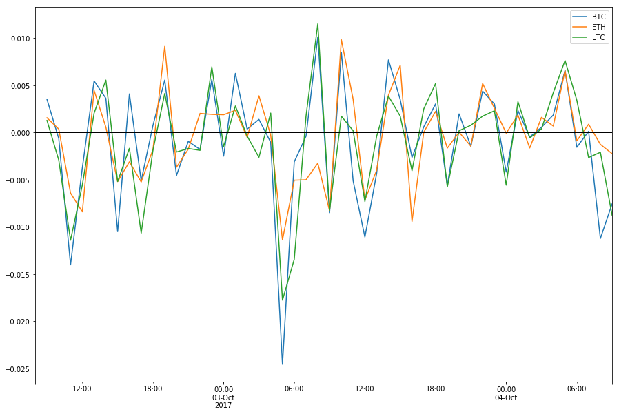
Visualize Log Returns
We plot normalized changes of closing prices for last 50 hours. Log differences can be interpreted as the percentage change.
df_change[:50].plot(figsize=(15, 10)).axhline(color='black', linewidth=2)
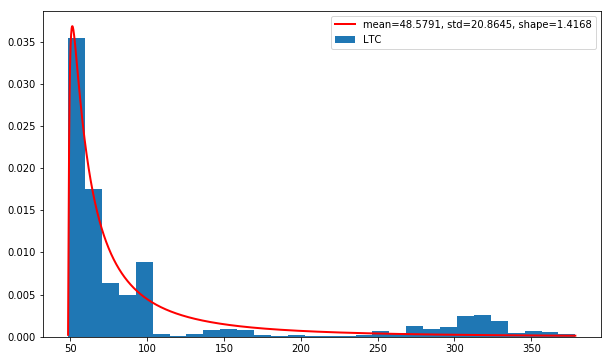
Are LTC prices distributed log-normally?
If we assume that prices are distributed log-normally, then $log(1 + r_i)$ is conveniently normally distributed (for details, see Why Log Returns)
On the chart below, we plot the distribution of LTC hourly closing prices. We also estimate parameters for log-normal distribution and plot estimated log-normal distribution with a red line.
from scipy.stats import lognorm
import matplotlib.pyplot as plt

fig, ax = plt.subplots(figsize=(10, 6))

values = df['LTC']

shape, loc, scale = stats.lognorm.fit(values)
x = np.linspace(values.min(), values.max(), len(values))
pdf = stats.lognorm.pdf(x, shape, loc=loc, scale=scale)
label = 'mean=%.4f, std=%.4f, shape=%.4f' % (loc, scale, shape)

ax.hist(values, bins=30, normed=True)
ax.plot(x, pdf, 'r-', lw=2, label=label)
ax.legend(loc='best')
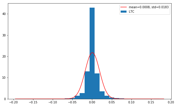
Are LTC log returns normally distributed?
On the chart below, we plot the distribution of LTC log returns. We also estimate parameters for normal distribution and plot estimated normal distribution with a red line.
import pandas as pd
import numpy as np
import scipy.stats as stats
import matplotlib.pyplot as plt

values = df_change['LTC'][1:]  # skip first NA value
x = np.linspace(values.min(), values.max(), len(values))

loc, scale = stats.norm.fit(values)
param_density = stats.norm.pdf(x, loc=loc, scale=scale)
label = 'mean=%.4f, std=%.4f' % (loc, scale)

fig, ax = plt.subplots(figsize=(10, 6))
ax.hist(values, bins=30, normed=True)
ax.plot(x, param_density, 'r-', label=label)
ax.legend(loc='best')
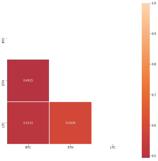
Pearson Correlation with log returns
We calculate Pearson Correlation from log returns. The correlation matrix below has similar values as the one at Sifr Data. There are differences because:
- we don’t calculate volume-weighted average daily prices
- different time period (hourly and daily),
- different data source (Coinbase and Poloniex).
Observations
- BTC and ETH have moderate positive relationship,
- LTC and ETH have strong positive relationship.
import seaborn as sns
import matplotlib.pyplot as plt

# Compute the correlation matrix
corr = df_change.corr()

# Generate a mask for the upper triangle
mask = np.zeros_like(corr, dtype=np.bool)
mask[np.triu_indices_from(mask)] = True

# Set up the matplotlib figure
f, ax = plt.subplots(figsize=(10, 10))

# Draw the heatmap with the mask and correct aspect ratio
sns.heatmap(corr, annot=True, fmt = '.4f', mask=mask, center=0, square=True, linewidths=.5)
Conclusion
We showed how to calculate log returns from raw prices with a practical example. This way we normalized prices, which simplifies further analysis. We also showed how to estimate parameters for normal and log-normal distributions.