5 mistakes when writing SQL queries
SQL is widely used for data analytics and data extraction. Although it is fairly easy to start with SQL, bugs can quickly sneak into the queries as I show with examples below.
These are 5 mistakes I did when writing SQL queries. Examples are short and may look simple, but when working on larger queries, these mistakes may not be obvious at first sight. Some of the examples are AWS Redshift specific, while others can occur with other SQL databases (Postgres, MySQL, etc.). These examples should run on your local database or you can run them online with SQL Fiddle.
Example SQL queries are available to download.

Here are a few links you might be interested in:
- Intro to Machine Learning
- Intro to Programming
- Data Science for Business Leaders
- AI for Healthcare
- Autonomous Systems
- Learn SQL
Disclosure: Bear in mind that some of the links above are affiliate links and if you go through them to make a purchase I will earn a commission. Keep in mind that I link courses because of their quality and not because of the commission I receive from your purchases. The decision is yours, and whether or not you decide to buy something is completely up to you.
Setup
Let’s create two temporary tables with few entries that will help us with examples.
Table sales
This table contains sales entries with the timestamp, product, price, etc. Note that the key column is unique, values in other columns can be repeated (eg. ts column).
DROP TABLE IF EXISTS sales;
CREATE TEMPORARY TABLE sales
(
    key       varchar(6),
    ts        timestamp,
    product   integer,
    completed boolean,
    price     float
);

INSERT INTO sales
VALUES ('sale_1', '2019-11-08 00:00', 0, TRUE, 1.1),
       ('sale_2', '2019-11-08 01:00', 0, FALSE, 1.2),
       ('sale_3', '2019-11-08 01:00', 0, TRUE, 1.3),
       ('sale_4', '2019-11-08 01:00', 1, FALSE, 1.4),
       ('sale_5', '2019-11-08 02:00', 1, TRUE, 1.5),
       ('sale_6', '2019-11-08 02:00', 1, TRUE, 1.5);
SELECT * FROM sales;
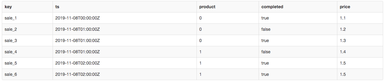
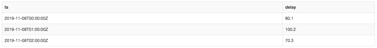
Table hourly delay
This table contains delays per hour for a certain day. Note that the ts column is unique in the table below.
DROP TABLE IF EXISTS hourly_delay;
CREATE TEMPORARY TABLE hourly_delay
(
    ts    timestamp,
    delay float
);


INSERT INTO hourly_delay
VALUES ('2019-11-08 00:00', 80.1),
       ('2019-11-08 01:00', 100.2),
       ('2019-11-08 02:00', 70.3);
SELECT * FROM hourly_delay;
1. Calculating the average of an integer column
Let’s calculate the average of a product column which has an integer type.
SELECT avg(product)
FROM sales;
There are three 0 and three 1 in the product column so we would expect the average to be 0.5. Most databases like the latest version of Postgres would return 0.5, but Redshift returns 0 because it doesn’t cast the product column to float automatically. We need to cast it to float type:
SELECT avg(product::FLOAT)
FROM sales;
2. Calculating average with conditions
Let’s calculate the average price of products where the sale was completed. The value we are looking for is (1.1 + 1.3 + 1.5 + 1.5) / 4, which is 1.35.
SELECT avg(price)
FROM (SELECT CASE WHEN completed = TRUE THEN price else 0 END AS price FROM sales) AS q1;
When we run the query, we get 0.9. Why is that? This happens: (1.1 + 0 + 1.3 + 0 + 1.5 + 1.5) / 6 is 0.9. The mistake in the query is that we set 0 to entries that shouldn’t be included. Let’s use NULL instead of 0.
SELECT avg(price)
FROM (SELECT CASE WHEN completed = TRUE THEN price else NULL END AS price FROM sales) AS q1;
Now the output is 1.35 as expected.
3. Ordering by the same timestamps
Let’s retrieve the price of the last sale for each product:
SELECT price
FROM (SELECT price, row_number() OVER (PARTITION BY product ORDER BY ts DESC) AS ix FROM sales) AS q1
WHERE ix = 1;
The problem with the query above is that there are multiple sales with the same timestamp. Consecutive runs of this query on the same data could return a different result. We can observe on the image below, that product 0 has two sales at 2019-11-08 01:00 with 1.2 and 1.3 prices.
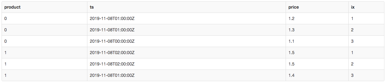
We are going to fix the query with the next mistake :)
4. Adding columns to ORDER BY
The fix for the mistake above is obvious. Let’s add the key column to ORDER BY and that will make the result of the query repeatable on the same data - a quick fix.
SELECT price
FROM (SELECT price, row_number() OVER (PARTITION BY product ORDER BY ts, key DESC) AS ix FROM sales) AS q1
WHERE ix = 1;

Why are the query results different from the previous run? When we were making “a quick fix”, we put the key column in the wrong place in the ORDER BY. It should be behind the DESC statement, not before it. Instead of the last sale, the query is now returning the first sale. Let’s do another fix.
SELECT product, price
FROM (SELECT product, price, row_number() OVER (PARTITION BY product ORDER BY ts DESC, key) AS ix FROM sales) AS q1
WHERE ix = 1;

This fix makes results repeatable.
5. Inner join
Let’s say we would like to sum all delays in sales per day and also calculate the average price of sales per day.
SELECT t2.ts::DATE, sum(t2.delay), avg(t1.price)
FROM hourly_delay AS t2
         INNER JOIN sales AS t1 ON t1.ts = t2.ts
GROUP BY t2.ts::DATE;

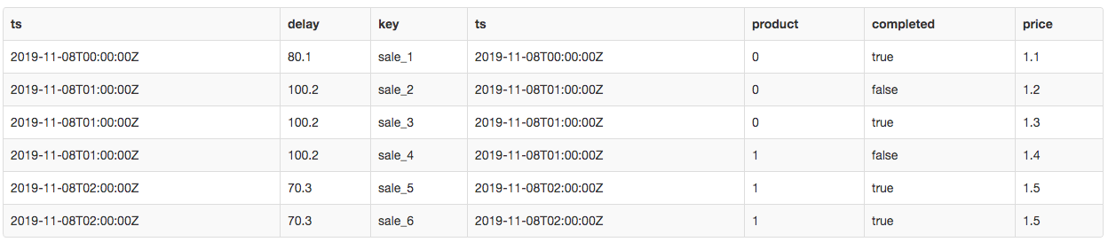
The result is wrong! The query above multiples the delay column from the hourly_delay table as can be seen in the image below. This happens because we join by timestamp, which is unique in the hourly_delay table, but it is repeated in the sales table.
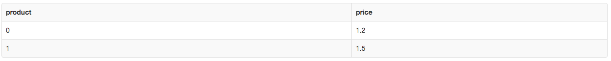
To fix the problem, we are going to calculate statistics for each table in a separate subquery and then join the aggregates. This makes timestamps unique in both tables.
SELECT t1.ts, daily_delay, avg_price
FROM (SELECT t2.ts::DATE, sum(t2.delay) AS daily_delay FROM hourly_delay AS t2 GROUP BY t2.ts::DATE) AS t2
         INNER JOIN (SELECT ts::DATE AS ts, avg(price) AS avg_price FROM sales GROUP BY ts::DATE) AS t1 ON t1.ts = t2.ts;

Conclusion
We went through a few common SQL mistakes and solutions. Do you have an interesting story with SQL queries? Let me know in the comments below.